Dynamic Stability of Children Gait

 

 

Dan B. Marghitu and Eleonor D. Stoenescu

 

Department of Mechanical Engineering, Auburn University, AL 36849, USA

 

 

Abstract.  In this study we used the techniques of nonlinear dynamics to analyze the stability of normal and pathological gait in children. We based the analysis on the assumption that a human at steady state locomotion can be represented as a nonlinear periodic system. Kinematic data for the lower limb joints were used to construct phase plane portraits for the hip, the knee and the ankle joints. Anomalies in the joint rotations of pathological individuals were graphically depicted, by comparing the phase plane portraits. Using the Floquet theory, an index of dynamic stability was used to compare normal and pathological gait.

 

1 Introduction

The study of human gait has been the culmination of numerous efforts in understanding the basic principles underlying this phenomenon. These studies have a direct application in the diagnosis of gait abnormalities and in their effective treatment. The methodologies adopted for carrying out these studies have diverse origins and have consistently evolved with developments in technology.

The first return map was used along with the phase plane portraits to distinguish gait abnormalities in humans [1]. Along with these techniques, a scalar measure that allowed for a comparison between the dynamic stability of normal and post-polio gait was proposed [2]. In this study we base our analysis on phase plane portraits, Poincaré maps and the Floquet multipliers [3]. We analyze the stability of walking in children both normal and with pathological disorders of the knee and ankle.

2 Human subjects and data collection

The study was carried out over a subject population of six children belonging to the age group of 7-9 years. One of the subjects was classified as being perfectly normal with no indications of any pathologic disorders. The remaining five subjects had pathologic rotational disorders of the knee or ankle joints to a varying degree.

3 Mathematical background

The walking human being can be then represented as a nonautonomous, periodically forced nonlinear dynamical system, by a set of n first order ordinary differential equations:

 

                                                                                                                     (1)

 

where x is a vector in the phase space <ⁿ. The vector field F(.,t) = F(.,t+T) is periodic in time with a period T. A set of solutions representing the walking patterns of the human would then be given by

 

                                                                 x(t) = x(t + T)                                                       (2)

 

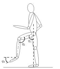
For the mathematical analysis of any such system, it is required to identify a set of variables that describe the dynamics of the system. For this purpose we consider the simplified planar model shown in Figure 1. For simplifying the analysis the joints are assumed to be purely rotational with non-deformable members. Rotations of the hip joint (q₁), the knee joint (q₂), the ankle joint (q₃) and their corresponding angular velocities  are selected as the variables of state. The vector x can then be represented as

 

                                                                                                          (3)

 

Fig. 1 The simplified planar model

The motion of this system would then evolve in 6-dimensional state space and the solutions can be studied by considering their trajectories in the  projections of this space. This task is complicated by the fact that time appears as an additional coordinate, since the system is nonautonomous. A simple way to overcome this difficulty is by using the method of the Poincaré sections. The technique involves placing fictitious planes transverse to the trajectories in phase space at regular intervals and observing the points of intersection. For further illustration, let us represent the trajectories of the system given by Eq. (1) as G. We define a hyperplane S such that a) it is always transverse to G and b) the trajectories always cross it in the same direction. Also let the points of intersection of G with S be represented by x₀, x₁, . . . , x_k, . . .. The Poincaré map would then be a continuous mapping M of S into itself, such that

 

                                                                                          (4)

 

As Eq. (1) has a unique solution, each intersecting point of G and S can be determined from the previous one. This would imply that a continuous-time evolution of Eq. (1) will be replaced with a discrete-time mapping, by the Poincaré section. To analyze the stability of these trajectories we insert the Poincaré sections at well defined instances of the gait cycle. For a human being in locomotion, each cycle would be defined as the motion achieved in between successive foot contact events of the same limb. A choice of events could be the heel strike, heel off, toe on and toe off or even the instant of maximum flexion of the knee joint. Choosing the instant of maximum flexion of knee joint for inserting the Poincaré map Eq. (1) can be represented by

 

                                                                                                                   (5)

 

where, the subscript kf denotes maximum knee flexion, x_k and x_k+1 represent the vector sampled at the instant of maximum knee flexion during the k^th and k + 1^th cycles respectively. The stability of the closed orbit can then be determined with respect to infinitesimal perturbations d. The Poincaré map M_kf is then linearized in the neighborhood of x_e and is described by

 

                                                                                                                     (6)

 

where the J is known as the Jacobian or the Floquet matrix. The stability of the above system can be studied by observing the eigenvalues of the Floquet matrix (represented by l_j, j = 1, 6). To visualize this idea in a better manner let us rewrite the above equation in a different form. The linearized system after one period can be represented as

 

                                                                                                          (7)

 

where the image of a point x_e + d which initially was in the neighborhood of x_e is now at a distance. After m periods the system is represented by the expression

 

                                                                                                       (8)

where the initial displacement d is multiplied by J^m . If the eigenvalues of J (also known as the Characteristic multipliers) are less than one in magnitude, then any displacement from the fixed point x_e decreases exponentially and the periodic trajectory is asymptotically stable. On the other hand if the magnitude of any of the eigenvalues is larger than one, the displacement would grow exponentially and the trajectory would be unstable. If we compare the gait of two subjects who have all their multipliers within the unit circle, the gait of the subject with the larger multiplier will be less stable than that of the other. Utilizing this property, we define a scalar measure of gait stability as,

 

                                                                                                  (9)

 

The system under consideration is a human being system and the analytical representations of the function M_kf and the matrix J are extremely difficult to obtain. However, we can estimate J from experimentally acquired kinematic data [1, 2] using curve fitting techniques. This estimation of J is then used to compute the g-measures.

4 Results

Fig. 2 Phase plane portraits for the subject with normal gait and the portraits for three of the subjects with pathological gait

Kinematic data of the hip joint (q₁), the knee joint (q₂) and the ankle joint (q₃) were defined in the saggital plane and collected using a video based motion analysis system for a minimum of 5 gait cycles. Each gait cycle was defined as the motion achieved between consecutive heel strike events of the same foot. The joint rotation data for all three joints were numerically differentiated to obtain the corresponding velocities and both quantities were averaged over the five cycles. Phase plane portraits for each joint were obtained by plotting these averaged joint rotations against their respective velocities. The instant of heel strike was also averaged and plotted on the phase plane portraits.

Figure 2 depicts phase plane portraits for the subject with normal gait along with the portraits for three of the subjects with pathological gait. The fact that all the phase trajectories on the portraits are closed loops indicates that the joint movements are periodic. The Floquet multipliers for the normal and pathological subjects were computed from the Jacobian matrix and depicted on the complex plane.

Fig. 3 Floquet multipliers on the complex plane

The multipliers for all subjects were less than one in magnitude. Relative stability of gait for all subjects was quantified by comparing the magnitudes of their largest multipliers, which was defined as the g measure. The g measure for the subject with normal gait had a value of 0.47. The measures for all the pathological subjects were compared with that of the normal and were found to vary from 0.55 to 0.78, Figure 3.

This would imply that the gait of all five pathological subjects is more unstable than the gait of the normal subject. Also the subject with a g measure of 0.78 has the most unstable gait as compared to all the other subjects.

 

References

[1]           Y. Hurmuzlu et al., “Presenting joint kinematics of human locomotion using phase plane portraits and the Poincaré maps”, J. Biomech. 27 (12), pp. 1495, 1994.

[2]           Y. Hurmuzlu and C. Basdogan, “On the measurement of stability in human locomotion”, J. Biomech. 116, 30 1994.

[3]           A. H. Nayfeh and B. Balachandran, Applied Nonlinear Dynamics, John Wiley & Sons, Inc., New York, 1995.